cfsem python examples¶

Field Explorer¶

In this interactive example, examine the B-field and A-field of cfsem's finite-length-finite-thickness filament calcs and compare to point-source calculations, section discretizations, and \(B = \nabla \times A\) equivalence tests.

The full example can be run like uv run --group dev examples/field_explorer.py; the plot shown below is only an excerpt.

B-field of an arrangement of finite-length, finite-thickness filaments.

Helmholtz Coil Pair¶

This example uses cfsem.flux_density_circular_filament to map the B-field of a Helmholtz coil pair, an arrangement of two circular coils which produces a region of nearly uniform magnetic field.

Helmholtz coil example — B-field of a Helmholtz coil, calculated with cfsem. On the left, the red dashes outline where the B-field magnitude is within 1% of its value at (r=0, z=0), and the black dots show where the coils intersect the r-z plane.

examples/helmholtz.py

"""Calculate the B-field from a Helmholtz coil pair."""

import os
import time
from pathlib import Path

import numpy as np

if os.getenv("CFSEM_TESTING"):
    import matplotlib

    matplotlib.use("Agg")

from matplotlib import pyplot as plt

from cfsem import MU_0, flux_density_circular_filament

coil_radius = 0.2  # [m]

# The helmholtz coil pair comprised two circular coils,
# separated by a distance equal to their radius.
# In our coordinate system, z = 0 is the midpoint between the coils.
rfil = [coil_radius, coil_radius]  # [m]
zfil = [-0.5 * coil_radius, 0.5 * coil_radius]  # [m]

# [A] The current * turns of each coil.
ifil = [100.0, 100.0]

# Define a mesh on which to evaluate the B-field.
# Note that we cannot evaluate the B-field at exactly r = 0.
r = np.linspace(1e-9, 2.0 * coil_radius, 100)  # [m]
z = np.linspace(-1.5 * coil_radius, 1.5 * coil_radius, 100)  # [m]
rmesh, zmesh = np.meshgrid(r, z)
rmesh_flat = rmesh.flatten()
zmesh_flat = zmesh.flatten()

# Calculate the B-field at every mesh point using cfsem.
t0 = time.perf_counter()
Br_flat, Bz_flat = flux_density_circular_filament(ifil, rfil, zfil, rmesh_flat, zmesh_flat)
elapsed = time.perf_counter() - t0
print(f"Computed Helmholtz coil field at {rmesh.size} locations in {elapsed:.6f} s")


Br = Br_flat.reshape(rmesh.shape)
Bz = Bz_flat.reshape(rmesh.shape)

Bmag = np.sqrt(Br**2 + Bz**2)  # [T] Magnitude of the B-field.

fig, axes = plt.subplots(1, 2, figsize=(8, 4))
ax_map, ax_center = axes
ax_map.set_aspect("equal")
# Plot magnetic field lines.
ax_map.streamplot(rmesh, zmesh, Br, Bz, color="black", linewidth=0.5)
# Make a color plot of the magnetic field magnitude.
dr = r[1] - r[0]
dz = z[1] - z[0]
extent = (r[0] - dr / 2, r[-1] + dr / 2, z[0] - dz / 2, z[-1] + dz / 2)
im = ax_map.imshow(
    Bmag, extent=extent, origin="lower", interpolation="bicubic", norm="log"
)
fig.colorbar(im, label="$|\\vec{B}|$ [T]", ax=ax_map)
# Outline the region where the B-field magnitude is within 1% of the center value.
B_center = (4 / 5) ** (3 / 2) * MU_0 * ifil[0] / coil_radius  # [T]
ax_map.contour(
    rmesh,
    zmesh,
    np.abs(Bmag - B_center),
    levels=[0.01 * B_center],
    colors=["red"],
    linestyles="dashed",
)
# Draw the location of the coils.
ax_map.plot(rfil, zfil, color="black", marker="o", markersize=8, linestyle="none")
ax_map.set_title("$(r, z)$ map of $\\vec{B}$")

ax_map.set_xlabel("$r$ [m]")
ax_map.set_ylabel("$z$ [m]")
ax_map.set_xlim(0.0, r[-1])
ax_map.set_ylim(z[0], z[-1])


# Plot the centerline B-field from cfsem versus the analytic solution.
# Analytic formula from https://en.wikipedia.org/wiki/Helmholtz_coil#Derivation
def xi(x):
    """Helper function for calculating the centerline B-field analytically."""
    return (1 + (x / coil_radius) ** 2) ** (-3 / 2)


Bmag_analytic = (
    MU_0 / (2 * coil_radius) * (ifil[0] * xi(z - zfil[0]) + ifil[1] * xi(z - zfil[1]))
)
ax_center.plot(
    z, Bz[:, 0], label="cfsem", marker="+", color="tab:blue", linestyle="none"
)
ax_center.plot(z, Bmag_analytic, label="analytic", color="black")
# Annotate the coil locations.
for i in (0, 1):
    ax_center.axvline(zfil[i], color="gray", linestyle="--")
    ax_center.text(
        s=f"coil {i + 1}",
        x=zfil[i],
        y=0.5 * np.max(Bmag_analytic),
        rotation=90,
        ha="right",
        va="center",
        color="grey",
    )
ax_center.axvline(zfil[1], color="gray", linestyle="--")
ax_center.set_xlabel("$z$ [m]")
ax_center.set_ylabel("$|\\vec{B}|$ [T]")
ax_center.legend(loc="lower right")
ax_center.set_ylim(0.0, 1.1 * np.max(Bmag_analytic))
ax_center.set_title("Centerline ($r=0$) $B$-field")

fig.tight_layout()
fpath = Path("__file__").parent / "helmholtz.png"
fig.savefig(fpath, dpi=300)

Quadrilateral Element Explorer¶

Explore quad4 and quad9 interpolation in a Plotly Dash app. The example shows a central element with one layer of neighboring elements, quadrature locations for gl3 or gl4, and the interpolated scalar field lifted above the analysis mesh.

Run it with uv run --group dev examples/element_explorer.py.

Quadrilateral interpolation surface and quadrature points.

High-aspect-ratio Coil Inductance¶

Estimate the (low-frequency) self- and mutual- inductance of a pair of air-core solenoids, comparing results from modeling as either collections of axisymmetric loops or as thin helical filaments.

examples/inductance.py

"""
Comparison of self- and mutual- inductance of coils modeled as either an axisymmetric filament collection
or as a piecewise-linear helix.
"""

import numpy as np

import cfsem

# Center radius and height, winding pack width and height,
# and number of windings in r and z directions
# for two solenoids.
r1, z1, w1, h1, nr1, nz1 = (0.3, 0.0, 0.01, 1.0, 1, 10)
r2, z2, w2, h2, nr2, nz2 = (0.5, 0.2, 0.01, 0.5, 1, 5)

cnd_w1, cnd_h1 = (0.02, 0.02)  # Approximate conductor width and height for first coil
cnd_w2, cnd_h2 = (0.02, 0.02)  # Approximate conductor width and height for second coil

nt1 = nr1 * nz1  # Total number of turns for each coil
nt2 = nr2 * nz2

# Build axisymmetric filament representation
filaments_1 = cfsem.filament_coil(r1, z1, w1, h1, nt1, nr1, nz1)
filaments_2 = cfsem.filament_coil(r2, z2, w2, h2, nt2, nr2, nz2)

# Build helix representations with 100 points per turn.
# The first and last point in the helices span the full height of the winding pack
# such that each filament in the axisymmetric representation captures a half turn
# of the helical representation above and below its z-location.
angles1 = np.linspace(0.0, 2.0 * np.pi * nt1, 100 * nt1)  # [rad]
angles2 = np.linspace(0.0, 2.0 * np.pi * nt2, 100 * nt2)  # [rad]

xhelix1 = r1 * np.cos(angles1)  # [m]
yhelix1 = r1 * np.sin(angles1)  # [m]
zhelix1 = np.linspace(z1 - h1 / 2, z1 + h1 / 2, angles1.size)  # [m]

xhelix2 = r2 * np.cos(angles2)  # [m]
yhelix2 = r2 * np.sin(angles2)  # [m]
zhelix2 = np.linspace(z2 - h2 / 2, z2 + h2 / 2, angles2.size)  # [m]

# Estimate the self-inductance by 2 different methods,
# hand-calc and helical filaments.
self_inductance_handcalc_1 = cfsem.self_inductance_lyle6(r1, w1, h1, nt1)
self_inductance_handcalc_2 = cfsem.self_inductance_lyle6(r2, w2, h2, nt2)

self_inductance_helical_1 = cfsem.self_inductance_piecewise_linear_filaments(
    (xhelix1, yhelix1, zhelix1),
    wire_radius=0.5 * cnd_w1,
)
self_inductance_helical_2 = cfsem.self_inductance_piecewise_linear_filaments(
    (xhelix2, yhelix2, zhelix2),
    wire_radius=0.5 * cnd_w2,
)

self_inductance_axisymmetric_1 = cfsem.self_inductance_axisymmetric_coil(
    f=filaments_1.T,
    section_kind="rectangular",
    section_size=(cnd_w1, cnd_h1),
)
self_inductance_axisymmetric_2 = cfsem.self_inductance_axisymmetric_coil(
    f=filaments_2.T,
    section_kind="rectangular",
    section_size=(cnd_w2, cnd_h2),
)

print("First coil self-inductance")
print(f"                Handcalc: {self_inductance_handcalc_1:.2e} [H]")
print(f"                 Helical: {self_inductance_helical_1:.2e} [H]")
print(f"            Axisymmetric: {self_inductance_axisymmetric_1:.2e} [H]")

print("Second coil self-inductance")
print(f"                Handcalc: {self_inductance_handcalc_2:.2e} [H]")
print(f"                 Helical: {self_inductance_helical_2:.2e} [H]")
print(f"            Axisymmetric: {self_inductance_axisymmetric_2:.2e} [H]")

# Estimate mutual inductance by 2 different methods,
# axisymmetric filaments and helical filaments.
mutual_inductance_axisymmetric = cfsem.mutual_inductance_of_cylindrical_coils(
    filaments_1.T, filaments_2.T
)
mutual_inductance_helical = cfsem.mutual_inductance_piecewise_linear_filaments(
    (xhelix1, yhelix1, zhelix1), (xhelix2, yhelix2, zhelix2)
)
#    Mutual inductance is reflexive, so we get the same answer if we reverse the inputs
mutual_inductance_axisymmetric_reflexive = cfsem.mutual_inductance_of_cylindrical_coils(
    filaments_2.T, filaments_1.T
)
mutual_inductance_helical_reflexive = (
    cfsem.mutual_inductance_piecewise_linear_filaments(
        (xhelix2, yhelix2, zhelix2), (xhelix1, yhelix1, zhelix1)
    )
)

print("Mutual-inductance")
print(f"            Axisymmetric: {mutual_inductance_axisymmetric:.2e} [H]")
print(f"                 Helical: {mutual_inductance_helical:.2e} [H]")
print(f"  Axisymmetric reflexive: {mutual_inductance_axisymmetric_reflexive:.2e} [H]")
print(f"       Helical reflexive: {mutual_inductance_helical_reflexive:.2e} [H]")

Axisymmetric FEM Solenoid Stress Explorer¶

Explore the axisymmetric FEM stress solver in a Plotly Dash app. The example varies the solenoid cross-section, current density, element family, quadrature, material model, and loop-source position. It assembles the sparse FEM system, adds the external loop source plus smooth winding-pack self-field, and compares radial sections against row-matched 1D finite-difference reference profiles.

Run it with uv run --group dev examples/solenoid_stress_axisymmetric_fem.py.

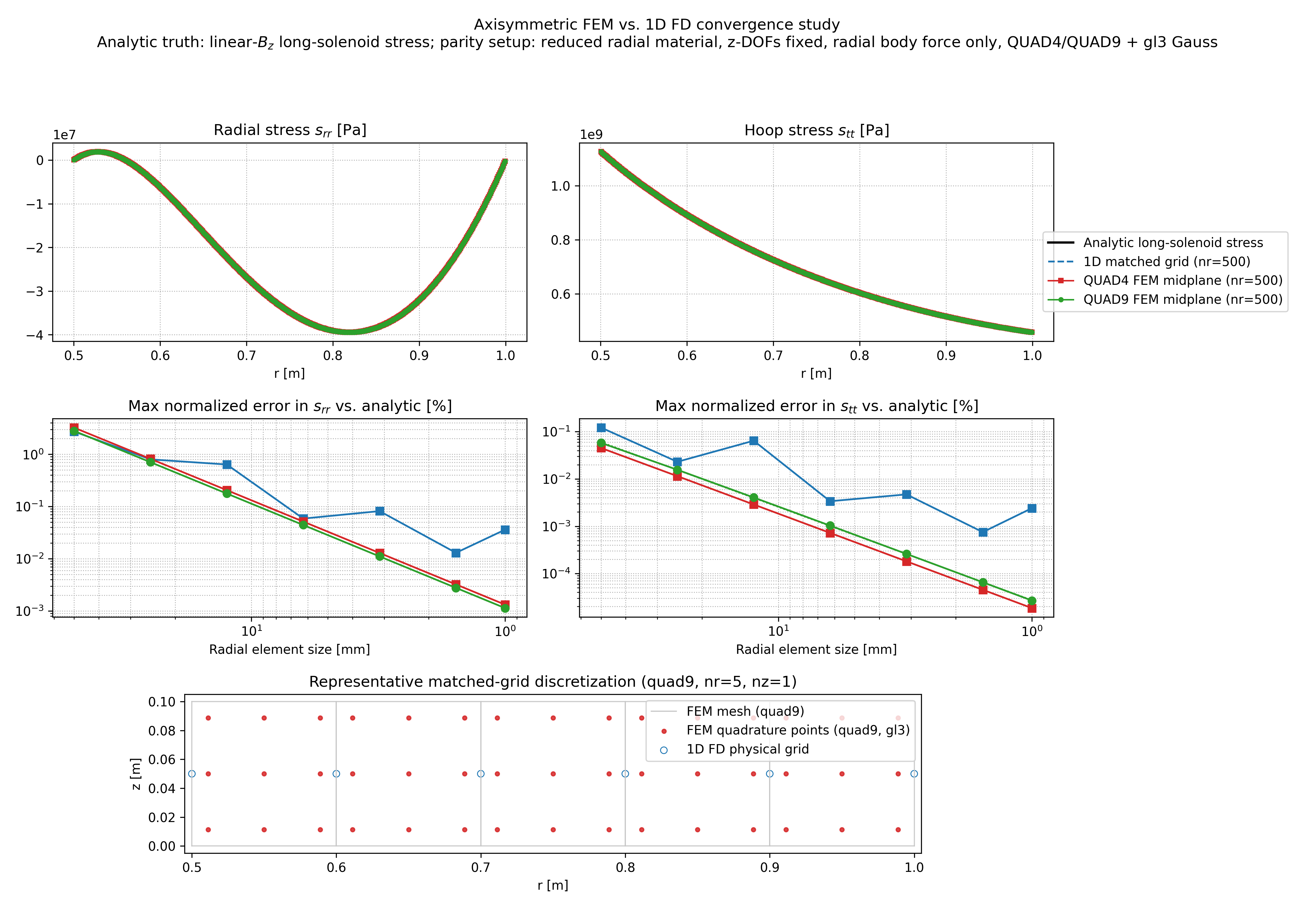
Axisymmetric FEM Solenoid Stress Convergence Study¶

Run an explicit radial-refinement study that configures the 2D FEM model to match the 1D solver assumptions as closely as possible, then compares both against the analytic long-solenoid stress formula on the midplane. The current hardcoded sweep uses quad9 elements with gl3 quadrature and radial target spacings from 50 mm down to 1 mm.

Run it with uv run --group dev examples/solenoid_stress_axisymmetric_fem_convergence.py or add --no-plot for CI-style execution.

Axisymmetric FEM convergence example — Midplane stress convergence for the 1D FD and axisymmetric FEM solenoid solvers.

Axisymmetric FEM Repeated-Load Operator Example¶

Run a small non-GUI example that assembles the constrained reduced model once, then updates the load values to rebuild the reduced right-hand side for multiple cases. The script makes the operator construction explicit, applies all four supported load types,

body-force density
surface pressure
surface traction in global (r, z) components
nodal temperature with thermal strain

and checks the Rust-side model.solve(rhs) result against a SciPy solve on the same reduced stiffness matrix. It uses the operators body_force_to_rhs, pressure_to_rhs, traction_to_rhs, temperature_to_rhs, and constant_rhs to rebuild the reduced load vector.

Run it with uv run --group dev examples/solenoid_stress_surface_traction.py.

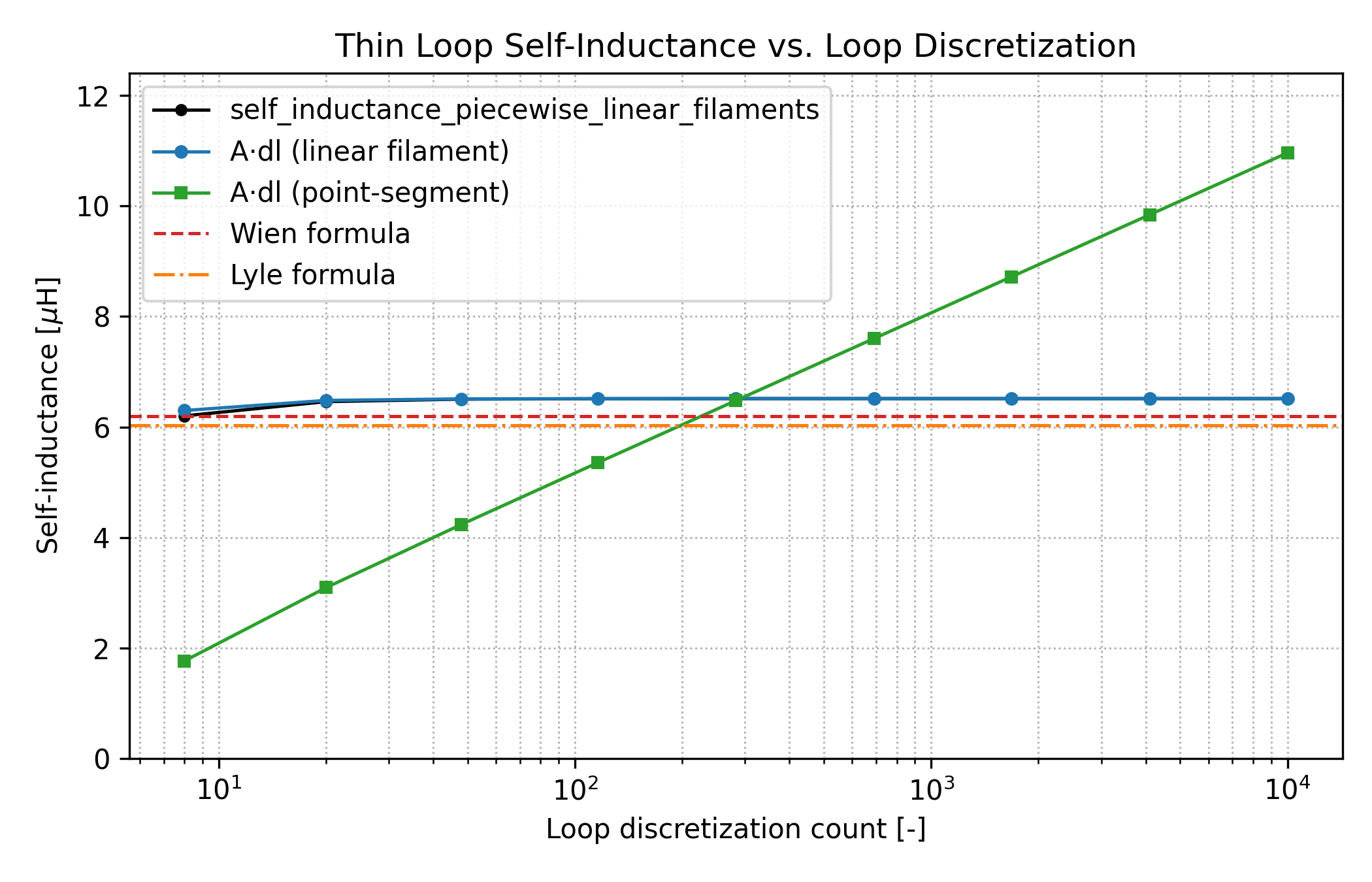
Loop Inductance¶

Estimate the (low-frequency) self-inductance of a finite-radius wire loop by different methods.